slacr_

Just to record my life and thoughts.
笔记/编程/杂乱/极简

[TensorFlow]实践

Jan 19, 2024ML5920 words in 39 min

TensorFlow assignment with AIGC

环境

Windows 11 23H2 希冀平台 VisualStudioCode 1.85.1 Python 3.9 TensorFlow2.9.0
Tensorflow-gpu 2.7.0 cudatoolkit11.8.0

深度学习与实践基础实验

图像增强

实现均值滤波

首先定义了一个 3x3 的均值滤波模板 kernel,它的每个元素都是 1/9,用于计算每个像素的均值。然后,使用 cv2.filter2D 函数将模板应用到图像上,得到均值滤波后的结果 output。
使用 cv2.cvtColor 函数将图像从 BGR 格式转换为 RGB 格式,因为 Matplotlib 默认使用 RGB 格式来显示图像。
最后,使用 plt.imshow 函数分别显示原始图像 img2 和均值滤波后的图像 output2。

1
2
3
4
5
6
7
8
9
10
11
12
13
14
15
16
17
18
19
20
21
22
23
24
25
26
27
28
29
30
31
32
33
import cv2
import numpy as np
import matplotlib.pyplot as plt

# 定义均值滤波模板
kernel = np.ones((3, 3), np.float32) / 9

# 读取图像
img = cv2.imread("ironman.jpg")

# 进行均值滤波
output = cv2.filter2D(img, -1, kernel)

# 将图像从 BGR 转换为 RGB 格式
img2 = cv2.cvtColor(img, cv2.COLOR_BGR2RGB)
output2 = cv2.cvtColor(output, cv2.COLOR_BGR2RGB)

# 创建一个包含两个子图的图像窗口
fig, axs = plt.subplots(1, 2, figsize=(10, 5))

# 在第一个子图中显示原始图像
axs[0].imshow(cv2.cvtColor(img, cv2.COLOR_BGR2RGB))
axs[0].set_title("Original Image")

# 在第二个子图中显示滤波后的图像
axs[1].imshow(cv2.cvtColor(output, cv2.COLOR_BGR2RGB))
axs[1].set_title("Filtered Image")

# 调整子图之间的间距
plt.tight_layout()

# 显示图像窗口
plt.show()

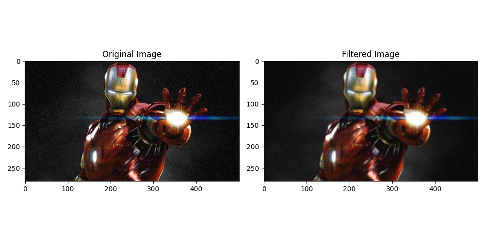
使用了均值滤波来处理了图像。均值滤波是一种常用的图像平滑处理方法,它可以减少图像中的噪声,并使图像变得更加模糊。
根据以上代码中的均值滤波模板(3x3 的全1矩阵除以9),我们可以看到滤波后的图像输出变得更加模糊。这是因为均值滤波将每个像素周围的邻域取平均值,从而减少了像素值之间的差异。

实现图像锐化

首先读取图像,并将其转换为灰度图像。定义了自己的Sobel算子,分别为x方向和y方向。接下来使用cv2.filter2D函数对灰度图像进行卷积计算,分别得到x方向和y方向的卷积结果。然后对卷积结果取绝对值并转换为8位图像。最后将x方向和y方向的卷积结果加权相加,得到最终的锐化图像。

1
2
3
4
5
6
7
8
9
10
11
12
13
14
15
16
17
18
19
20
21
22
23
24
25
26
27
28
29
30
31
32
33
34
35
36
37
38
39
40
41
42
import cv2
import numpy as np
import matplotlib.pyplot as plt

# 读取图像
img = cv2.imread("ironman.jpg")
lenna_img = cv2.cvtColor(img, cv2.COLOR_BGR2RGB)

# 灰度化处理图像
grayImage = cv2.cvtColor(img, cv2.COLOR_BGR2GRAY)

# 自定义Sobel算子
sobel_x = np.array([[-1, 0, 1], [-2, 0, 2], [-1, 0, 1]])
sobel_y = np.array([[-1, -2, -1], [0, 0, 0], [1, 2, 1]])

# 对x和y方向进行卷积计算
sobel_x_img = cv2.filter2D(grayImage, -1, sobel_x)
sobel_y_img = cv2.filter2D(grayImage, -1, sobel_y)

# 将卷积结果取绝对值并转换为8位图像
sobel_x_abs = cv2.convertScaleAbs(sobel_x_img)
sobel_y_abs = cv2.convertScaleAbs(sobel_y_img)

# 将x和y方向的卷积结果加权相加
sobel_result = cv2.addWeighted(sobel_x_abs, 0.5, sobel_y_abs, 0.5, 0)

# 创建一个包含两个子图的图像窗口
fig, axs = plt.subplots(1, 2, figsize=(10, 5))

# 在第一个子图中显示原始图像
axs[0].imshow(lenna_img)
axs[0].set_title("Original Image")

# 在第二个子图中显示锐化后的图像
axs[1].imshow(sobel_result, cmap="gray")
axs[1].set_title("Sharpened Image")

# 调整子图之间的间距
plt.tight_layout()

# 显示图像窗口
plt.show()

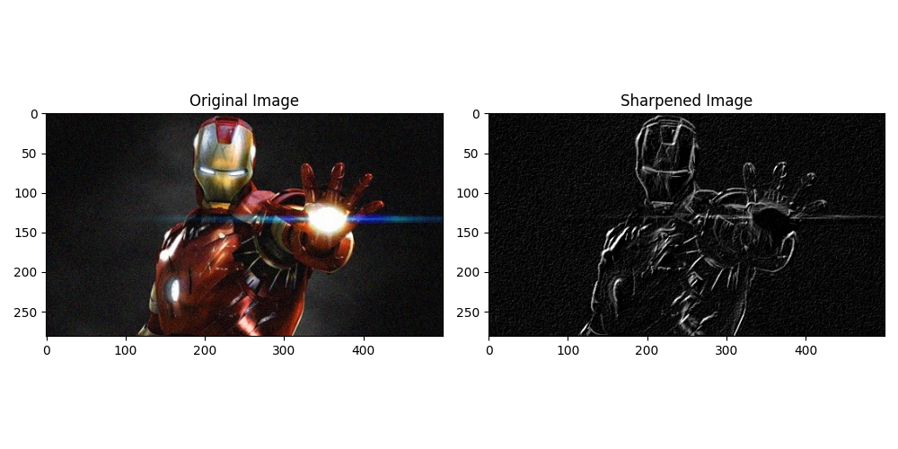
在上述代码中,我使用了自定义的Sobel算子来对图像进行锐化处理。Sobel算子是一种常用的边缘检测算子,它可以通过计算图像中每个像素点的梯度值来检测图像中的边缘。
通过观察锐化后的图像,看到图像的边缘得到了突出,并且图像的细节更加清晰。锐化图像可以用于增强图像的边缘和细节,使图像更加鲜明和有视觉冲击力。

基于TensorFlow卷积神经网络MNIST手写体数字图像分类

使用TensorFlow中的Keras API构建了一个简单的卷积神经网络(CNN)模型。模型包含了一个卷积层、一个池化层、一个Flatten层、一个全连接层和一个输出层。它使用adam优化器和sparse_categorical_crossentropy损失函数进行模型的编译,并使用训练集对模型进行了5个epoch的训练, 最后进行相应测试并输出图像结果。

1
2
3
4
5
6
7
8
9
10
11
12
13
14
15
16
17
18
19
20
21
22
23
24
25
26
27
28
29
30
31
32
33
34
35
36
37
38
39
40
41
42
43
44
45
46
47
48
49
50
51
52
53
54
55
56
57
58
59
60
61
62
63
64
65
66
67
import tensorflow as tf
import matplotlib.pyplot as plt
import numpy as np

# 下载MNIST数据集
mnist = tf.keras.datasets.mnist

# 加载数据集
(X_train, y_train), (X_test, y_test) = mnist.load_data()

# 数据预处理
X_train = X_train.reshape(-1, 28, 28, 1).astype(np.float32) / 255.0
X_test = X_test.reshape(-1, 28, 28, 1).astype(np.float32) / 255.0

# 检查是否已经有保存的模型
try:
model = tf.keras.models.load_model('p4_mnist_model.h5')
except:
# 如果没有保存的模型,则重新构建模型并进行训练
model = tf.keras.models.Sequential([
tf.keras.layers.Conv2D(32, (3, 3), activation='relu', input_shape=(28, 28, 1)),
tf.keras.layers.MaxPooling2D((2, 2)),
tf.keras.layers.Flatten(),
tf.keras.layers.Dense(64, activation='relu'),
tf.keras.layers.Dense(10, activation='softmax')
])

# 编译模型
model.compile(optimizer='adam',
loss='sparse_categorical_crossentropy',
metrics=['accuracy'])

# 训练模型
model.fit(X_train, y_train, epochs=5, validation_data=(X_test, y_test))

# 保存模型到文件
model.save('p4_mnist_model.h5')


# 创建包含多个子图的图像
num_tests = 5 # 设置要进行的测试次数
fig, axes = plt.subplots(1, num_tests, figsize=(12, 3))

for i in range(num_tests):
# 选择测试图像
index = i # 选择测试图像的索引
test_image = X_test[index]
test_label = y_test[index]

# 预测测试图像的类别
prediction = model.predict(np.expand_dims(test_image, axis=0))
predicted_label = np.argmax(prediction)

# 输出测试结果
print('True label:', test_label)
print('Predicted label:', predicted_label)

# 在子图中显示测试图像
axes[i].imshow(test_image.squeeze(), cmap='gray')
axes[i].axis('off')

# 在子图中添加标题,显示测试结果信息
title = f'True: {test_label}\nPredicted: {predicted_label}'
axes[i].set_title(title)

plt.tight_layout()
plt.show()

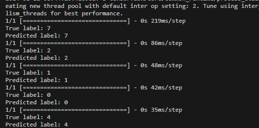
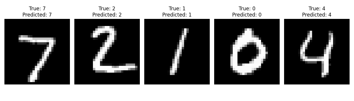
代码使用卷积神经网络模型对手写数字进行分类,并将预测结果可视化显示出来。我们可以看到每个测试图像的真实标签和模型预测的标签, 模型预测结果与真实结果相符合。

深度学习与实践进阶实验

基于无监督自编码器的图像去噪

基于TensorFlow搭建自动编码器对fashion_minist或minist数据集进行图像去噪,展示去噪前后的图像以及损失变化曲线。

首先加载fashion_mnist数据集,并进行了数据预处理,将像素值归一化到0-1之间,并将图像展平为一维向量。
接下来,定义了一个自动编码器模型,其中包含了编码器和解码器部分。编码器部分将输入图像压缩为低维表示,解码器部分将低维表示解码为重构图像。模型使用adam优化器和二进制交叉熵损失函数进行编译。
然后,使用带噪声的训练数据对自动编码器进行训练。训练过程中使用了回调函数来保存最佳模型和提前停止训练。
训练完成后,加载最佳模型并对带噪声的测试数据进行去噪。将去噪前后的图像进行可视化展示。
最后,绘制训练过程中的损失变化曲线。

1
2
3
4
5
6
7
8
9
10
11
12
13
14
15
16
17
18
19
20
21
22
23
24
25
26
27
28
29
30
31
32
33
34
35
36
37
38
39
40
41
42
43
44
45
46
47
48
49
50
51
52
53
54
55
56
57
58
59
60
61
62
63
64
65
66
67
68
69
70
71
72
73
74
75
76
77
78
79
80
81
82
83
84
85
86
87
88
89
90
91
92
93
94
95
96
97
98
import numpy as np
import matplotlib.pyplot as plt
from tensorflow.keras.layers import Input, Dense
from tensorflow.keras.models import Model
from tensorflow.keras.datasets import fashion_mnist
from tensorflow.keras.callbacks import ModelCheckpoint, EarlyStopping
from tensorflow.keras import regularizers

# 加载数据集
(x_train, _), (x_test, _) = fashion_mnist.load_data()

# 数据预处理
x_train = x_train.astype('float32') / 255.
x_test = x_test.astype('float32') / 255.
x_train = np.reshape(x_train, (len(x_train), 784))
x_test = np.reshape(x_test, (len(x_test), 784))

# 添加噪声
noise_factor = 0.4
x_train_noisy = x_train + noise_factor * np.random.normal(loc=0.0, scale=1.0, size=x_train.shape)
x_test_noisy = x_test + noise_factor * np.random.normal(loc=0.0, scale=1.0, size=x_test.shape)
x_train_noisy = np.clip(x_train_noisy, 0., 1.)
x_test_noisy = np.clip(x_test_noisy, 0., 1.)

# 定义自动编码器模型
input_img = Input(shape=(784,))
encoded = Dense(128, activation='relu')(input_img)
encoded = Dense(64, activation='relu')(encoded)
encoded = Dense(32, activation='relu')(encoded)
decoded = Dense(64, activation='relu')(encoded)
decoded = Dense(128, activation='relu')(decoded)
decoded = Dense(784, activation='sigmoid')(decoded)

autoencoder = Model(input_img, decoded)
autoencoder.compile(optimizer='adam', loss='binary_crossentropy')

# 训练自动编码器
checkpointer = ModelCheckpoint(filepath='model.weights.best.hdf5', verbose=2, save_best_only=True)
earlystopper = EarlyStopping(monitor='val_loss', patience=2, verbose=2, mode='auto')

history = autoencoder.fit(x_train_noisy, x_train,
epochs=50,
batch_size=256,
shuffle=True,
validation_data=(x_test_noisy, x_test),
callbacks=[checkpointer, earlystopper])

# 加载最佳模型
autoencoder = Model(input_img, decoded)
autoencoder.load_weights('model.weights.best.hdf5')

# 进行去噪
decoded_imgs = autoencoder.predict(x_test_noisy)

# 显示去噪前后的图像
plt.figure(figsize=(20, 12))
for i in range(10):
# 原图
ax = plt.subplot(3, 10, i + 1)
plt.imshow(x_test[i].reshape(28, 28))
plt.gray()
ax.get_xaxis().set_visible(False)
ax.get_yaxis().set_visible(False)
if i == 0:
ax.set_title('Original')
ax.set_ylabel('Original', rotation=0, labelpad=40)

# 加噪
ax = plt.subplot(3, 10, i + 11)
plt.imshow(x_test_noisy[i].reshape(28, 28))
plt.gray()
ax.get_xaxis().set_visible(False)
ax.get_yaxis().set_visible(False)
if i == 0:
ax.set_title('Noisy')
ax.set_ylabel('Noisy', rotation=0, labelpad=40)

# 降噪
ax = plt.subplot(3, 10, i + 21)
plt.imshow(decoded_imgs[i].reshape(28, 28))
plt.gray()
ax.get_xaxis().set_visible(False)
ax.get_yaxis().set_visible(False)
if i == 0:
ax.set_title('Denoised')
ax.set_ylabel('Denoised', rotation=0, labelpad=40)

plt.subplots_adjust(wspace=0.05, hspace=0.4)
plt.show()

# 显示损失变化曲线
plt.plot(history.history['loss'])
plt.plot(history.history['val_loss'])
plt.title('Model Loss')
plt.ylabel('Loss')
plt.xlabel('Epoch')
plt.legend(['Train', 'Validation'], loc='upper right')
plt.show()

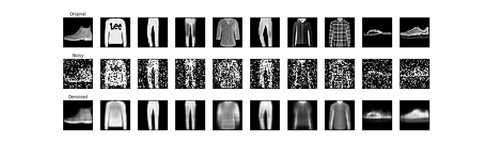
可以观察到自动编码器是如何去除加噪图像中的噪声并恢复原始图像的细节。

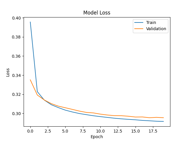
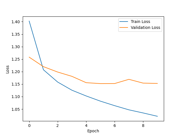
两者之间的差异很小,模型具有良好的泛化能力。训练损失和验证损失都随着训练的进行而下降,模型正在学习并逐渐改善。损失曲线平稳下降,说明模型在学习过程中相对稳定。

基于深度卷积神经网络的迁移学习

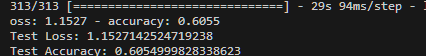
  • 不使用迁移学习, 直接训练一个新的神经网络, 计算测试集上的准确率

代码使用了一个简单的卷积神经网络模型来进行CIFAR-10的图像分类。首先加载CIFAR-10数据集,然后进行数据预处理,将像素值缩放到0到1之间。接下来构建模型,包括多个卷积层和全连接层。然后编译模型,指定优化器、损失函数和评估指标。最后使用训练集对模型进行训练,并使用测试集评估模型性能。

1
2
3
4
5
6
7
8
9
10
11
12
13
14
15
16
17
18
19
20
21
22
23
24
25
26
27
28
29
30
31
32
33
34
35
36
37
38
39
40
41
42
43
44
45
46
47
import tensorflow as tf
from tensorflow.keras.datasets import cifar10
from tensorflow.keras.models import Sequential
from tensorflow.keras.layers import Dense, Flatten, Conv2D, MaxPooling2D
from tensorflow.keras.models import load_model
import matplotlib.pyplot as plt

# 加载CIFAR-10数据集
(x_train, y_train), (x_test, y_test) = cifar10.load_data()

# 数据预处理
x_train = x_train / 255.0
x_test = x_test / 255.0

# 构建模型
model = Sequential()
model.add(Conv2D(32, (3, 3), activation='relu', input_shape=(32, 32, 3)))
model.add(MaxPooling2D((2, 2)))
model.add(Conv2D(64, (3, 3), activation='relu'))
model.add(MaxPooling2D((2, 2)))
model.add(Conv2D(64, (3, 3), activation='relu'))
model.add(Flatten())
model.add(Dense(64, activation='relu'))
model.add(Dense(10))

# 编译模型
model.compile(optimizer='adam',
loss=tf.keras.losses.SparseCategoricalCrossentropy(from_logits=True),
metrics=['accuracy'])

# 训练模型
history = model.fit(x_train, y_train, epochs=10, validation_data=(x_test, y_test))
model.save('cifar10_model.h5')

5
# 评估模型性能
test_loss, test_accuracy = model.evaluate(x_test, y_test)
print('Test Loss:', test_loss)
print('Test Accuracy:', test_accuracy)

# 显示损失曲线
plt.plot(history.history['loss'], label='Train Loss')
plt.plot(history.history['val_loss'], label='Validation Loss')
plt.xlabel('Epoch')
plt.ylabel('Loss')
plt.legend()
plt.show()

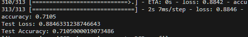
验证损失和训练损失之间的差值逐渐增大时,模型过拟合数据, 在未见过的新数据上的表现较差。能是由于模型的复杂性过高, 训练量过少。

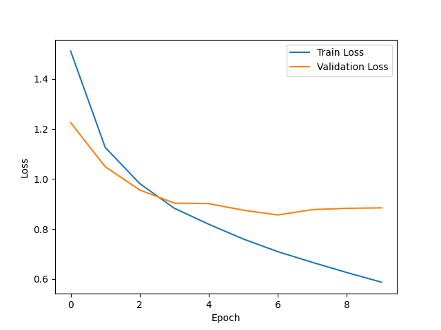
  • 使用VGG16模型和相同的数据集、参数进行迁移学习,计算测试集上的准确率
1
2
3
4
5
6
7
8
9
10
11
12
13
14
15
16
17
18
19
20
21
22
23
24
25
26
27
28
29
30
31
32
33
34
35
36
37
38
39
40
41
import tensorflow as tf
from tensorflow.keras.datasets import cifar10
from tensorflow.keras.applications import VGG16
from tensorflow.keras.models import Sequential
from tensorflow.keras.layers import Dense, Flatten
from tensorflow.keras.optimizers import Adam
import matplotlib.pyplot as plt

# 加载CIFAR-10数据集并进行预处理
(x_train, y_train), (x_test, y_test) = cifar10.load_data()
x_train = x_train / 255.0
x_test = x_test / 255.0

# 加载预训练的VGG16模型作为基础模型
base_model = VGG16(weights='imagenet', include_top=False, input_shape=(32, 32, 3))

# 冻结基础模型的权重
base_model.trainable = False

# 构建模型
model = Sequential()
model.add(base_model)
model.add(Flatten())
model.add(Dense(64, activation='relu'))
model.add(Dense(10, activation='softmax'))

# 编译模型
model.compile(optimizer=Adam(),
loss=tf.keras.losses.SparseCategoricalCrossentropy(from_logits=True),
metrics=['accuracy'])

# 记录训练过程中的损失值
history = model.fit(x_train, y_train, epochs=10, validation_data=(x_test, y_test))

# 绘制损失曲线
plt.plot(history.history['loss'], label='Train Loss')
plt.plot(history.history['val_loss'], label='Validation Loss')
plt.xlabel('Epoch')
plt.ylabel('Loss')
plt.legend()
plt.show()

损失曲线有起伏,在训练过程中损失值出现波动,模型在训练过程中难以收敛。对比可以发现,本次实验不使用迁移学习的准确率较高,可能是因为模型的架构或参数选择不合适。

基于深度学习的图像风格迁移

使用基于TensorFlow利用预训练的深度卷积网络(VGG19)完成图像风格迁移。

1
2
3
4
5
6
7
8
9
10
11
12
13
14
15
16
17
18
19
20
21
22
23
24
25
26
27
28
29
30
31
32
33
34
35
36
37
38
39
40
41
42
43
44
45
46
47
48
49
50
51
52
53
54
55
56
57
58
59
60
61
62
63
64
65
66
67
68
69
70
71
72
73
74
75
76
77
78
79
80
81
82
83
84
85
86
87
88
89
90
91
92
93
94
95
96
97
98
99
100
101
102
103
104
105
106
107
108
109
110
111
112
113
114
115
116
117
118
119
120
121
122
123
124
125
126
127
128
129
130
131
132
133
134
135
136
137
138
139
140
141
142
143
144
145
146
import tensorflow as tf
from tensorflow.keras.applications import vgg19
from tensorflow.keras.preprocessing.image import load_img, img_to_array
from tensorflow.keras.models import Model
import numpy as np
import matplotlib.pyplot as plt
from IPython import display
from PIL import Image

# 加载图像
def load_and_process_image(image_path):
img = load_img(image_path)
img = img_to_array(img)
img = np.expand_dims(img, axis=0)
img = vgg19.preprocess_input(img)
return img

# 反向处理图像,用于显示
def deprocess_image(x):
x = x.reshape((x.shape[1], x.shape[2], 3))
x[:, :, 0] += 103.939
x[:, :, 1] += 116.779
x[:, :, 2] += 123.68
# 'BGR'->'RGB'
x = x[:, :, ::-1]
x = np.clip(x, 0, 255).astype('uint8')
return x

# 计算内容损失
def content_loss(base_content, target):
return tf.reduce_mean(tf.square(base_content - target))

# 计算风格损失
def gram_matrix(input_tensor):
# print("Shape of input_tensor: ", input_tensor.shape)
# 将输入的形状调整为[height*width, channels]
input_tensor = tf.reshape(input_tensor, [-1, input_tensor.shape[-1]])
result = tf.matmul(input_tensor, input_tensor, transpose_a=True)
return result

def style_loss(style, target):
# print("Shape of style: ", style.shape)
# print("Shape of target: ", target.shape)
gram_style = gram_matrix(style)
gram_target = gram_matrix(target)
return tf.reduce_mean(tf.square(gram_style - gram_target))

# 加载预训练的VGG19模型
vgg = vgg19.VGG19(include_top=False, weights='imagenet')
vgg.trainable = False

# 选择中间层的输出以表示风格和内容
content_layers = ['block5_conv2']
style_layers = ['block1_conv1', 'block2_conv1', 'block3_conv1', 'block4_conv1', 'block5_conv1']

num_content_layers = len(content_layers)
num_style_layers = len(style_layers)

# 建立模型
def get_model():
vgg = vgg19.VGG19(include_top=False, weights='imagenet')
vgg.trainable = False
style_outputs = [vgg.get_layer(name).output for name in style_layers]
content_outputs = [vgg.get_layer(name).output for name in content_layers]
model_outputs = style_outputs + content_outputs
return Model(vgg.input, model_outputs)

# 定义风格和内容的权重
style_weight = 1e-2
content_weight = 1e4

# 定义优化器
opt = tf.optimizers.Adam(learning_rate=5)

# 定义训练步骤
@tf.function()
def train_step(image, model, optimizer, content_targets, style_targets):
with tf.GradientTape() as tape:
outputs = model(image)
content_outputs = outputs[num_style_layers:]
style_outputs = outputs[:num_style_layers]
style_score = 0
content_score = 0
weight_per_style_layer = 1.0 / float(num_style_layers)
for target_style, comb_style in zip(style_targets, style_outputs):
style_score += weight_per_style_layer * style_loss(comb_style[0], target_style)
weight_per_content_layer = 1.0 / float(num_content_layers)
for target_content, comb_content in zip(content_targets, content_outputs):
content_score += weight_per_content_layer * content_loss(comb_content[0], target_content)
loss = style_score * style_weight + content_score * content_weight
grads = tape.gradient(loss, image)
optimizer.apply_gradients([(grads, image)])
image.assign(tf.clip_by_value(image, 0, 255))
return loss

# 训练模型
def train_model(content_path, style_path, epochs=10, steps_per_epoch=500):
model = get_model()
for layer in model.layers:
layer.trainable = False

# 直接从文件中加载原始图像
content_image_orig = np.array(Image.open(content_path))
style_image_orig = np.array(Image.open(style_path))

# 将原始图像转换为预处理后的格式
content_image = load_and_process_image(content_path)
style_image = load_and_process_image(style_path)

images = [content_image_orig, style_image_orig] # 先添加原始的内容图像和风格图像
content_outputs = model(content_image)
style_outputs = model(style_image)
content_targets = content_outputs[num_style_layers:]
style_targets = style_outputs[:num_style_layers]
image = tf.Variable(content_image)
labels = ['Content Image', 'Style Image'] # 对应的标签
losses = [] # 用于保存每个epoch的损失值
for i in range(epochs):
for j in range(steps_per_epoch):
loss = train_step(image, model, opt, content_targets, style_targets)
print('.', end='')
display.clear_output(wait=True)
img = deprocess_image(image.numpy())
images.append(img) # 将生成的图像添加到列表中
labels.append('Epoch {}'.format(i+1)) # 添加对应的标签
losses.append(loss)

# 训练结束后,显示所有的图像
plt.figure(figsize=(20, 20))
for i, img in enumerate(images):
plt.subplot(len(images)//2 + len(images)%2, 2, i+1) # 修改为n行2列
plt.imshow(np.squeeze(img))
plt.title(labels[i]) # 显示对应的标签
plt.axis('off')
plt.show()
# 训练结束后,绘制损失曲线
plt.figure(figsize=(10, 5))
plt.plot(losses)
plt.title('Training Loss')
plt.xlabel('Epoch')
plt.ylabel('Loss')
plt.show()
return image

# 使用训练模型
final_image = train_model('content.jpg', 'style.jpg')

这段代码首先加载并预处理内容图像和风格图像,然后使用预训练的VGG19模型提取这些图像的特征。接着将内容图像作为初始图像,并在每个训练步骤中,根据内容损失和风格损失来更新这个图像。在训练过程中,会保存每个epoch的生成图像和损失值。最后展示内容图像、风格图像,以及训练中不同迭代次数的图像, 并绘制损失曲线。

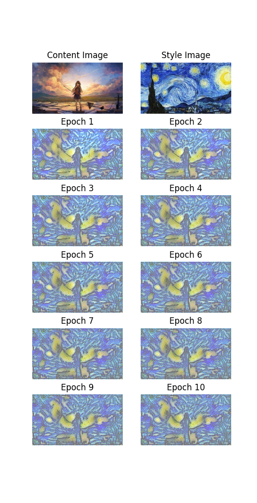
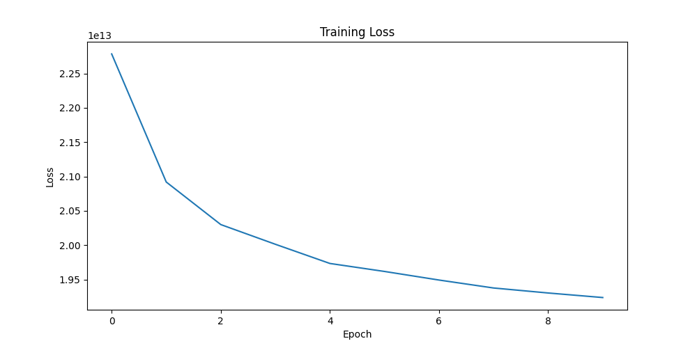
可以看到在steps_per_epoch为500, 共10个epoch的情况下,每次迭代生成的图像会逐渐接近目标风格,并保留内容图像的特征。平均损失曲线逐渐下降并趋于稳定,表示模型正在有效地学习从内容图像到目标风格的转换。

深度学习与实践创新实验

基于TensorFlow搭建卷积神经网络进行花卉图像分类

本次使用的数据集是来自Kaggle的Flowers Recognition数据集,包含了5种不同类型的花朵:雏菊(daisy)、蒲公英(dandelion)、玫瑰(rose)、向日葵(sunflower)和郁金香(tulip)。每种花朵都有多张图片,图片的大小和形状各不相同。
我使用ImageDataGenerator对花朵图片数据集进行预处理和数据增强,创建卷积神经网络模型用于花卉分类任务。模型训练完成后,保存模型并绘制训练和验证的损失和精度曲线。
训练好保存的模型之后会用于应用程序。

1
2
3
4
5
6
7
8
9
10
11
12
13
14
15
16
17
18
19
20
21
22
23
24
25
26
27
28
29
30
31
32
33
34
35
36
37
38
39
40
41
42
43
44
45
46
47
48
49
50
51
52
53
54
55
56
57
58
59
60
61
62
63
64
65
66
67
68
69
70
71
72
73
74
75
76
77
78
79
import tensorflow as tf
from tensorflow.keras.preprocessing.image import ImageDataGenerator
import matplotlib.pyplot as plt
# 加载数据集
data_dir = 'flowers'
image_size = (150, 150)
batch_size = 32


# 使用ImageDataGenerator来预处理图像并应用数据增强
datagen = ImageDataGenerator(
rescale=1./255,
validation_split=0.2,
rotation_range=40,
width_shift_range=0.2,
height_shift_range=0.2,
shear_range=0.2,
zoom_range=0.2,
horizontal_flip=True,
fill_mode='nearest'
)


train_generator = datagen.flow_from_directory(
data_dir,
target_size=image_size,
batch_size=batch_size,
class_mode='categorical',
subset='training'
)

validation_generator = datagen.flow_from_directory(
data_dir,
target_size=image_size,
batch_size=batch_size,
class_mode='categorical',
subset='validation'
)

# 创建卷积神经网络模型
model = tf.keras.models.Sequential([
tf.keras.layers.Conv2D(32, (3, 3), activation='relu', input_shape=(150, 150, 3)),
tf.keras.layers.MaxPooling2D((2, 2)),
tf.keras.layers.Conv2D(64, (3, 3), activation='relu'),
tf.keras.layers.MaxPooling2D((2, 2)),
tf.keras.layers.Conv2D(128, (3, 3), activation='relu'),
tf.keras.layers.MaxPooling2D((2, 2)),
tf.keras.layers.Flatten(),
tf.keras.layers.Dense(512, activation='relu'),
tf.keras.layers.Dense(5, activation='softmax')
])

# 编译模型
model.compile(loss='categorical_crossentropy', optimizer='adam', metrics=['accuracy'])

# 训练模型
history = model.fit(train_generator, validation_data=validation_generator, epochs=10)

# 保存模型
model.save('flowers_model.h5')


# 绘制训练损失和验证损失
plt.figure(figsize=(12, 4))
plt.subplot(1, 2, 1)
plt.plot(history.history['loss'], label='Train Loss')
plt.plot(history.history['val_loss'], label='Validation Loss')
plt.title('Losses')
plt.legend()

# 绘制训练精度和验证精度
plt.subplot(1, 2, 2)
plt.plot(history.history['accuracy'], label='Train Accuracy')
plt.plot(history.history['val_accuracy'], label='Validation Accuracy')
plt.title('Accuracies')
plt.legend()

plt.tight_layout()
plt.show()

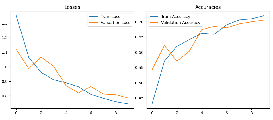
损失曲线在不断下降,准确度不断上升, 模型较稳定可靠。

我写了一个基于PyQt5的桌面应用,使用上文预训练的TensorFlow模型来对用户选择的花朵图片进行分类。在用户界面中,用户可以点击按钮选择图片,然后应用程序会显示选中的图片,并使用模型预测图片中花朵的种类。预测结果会显示在界面上。在后台,应用程序首先加载预训练的模型,然后在用户选择图片后,将图片调整到模型需要的尺寸,然后将图片转换为模型可以处理的数组格式,最后使用模型进行预测。

1
2
3
4
5
6
7
8
9
10
11
12
13
14
15
16
17
18
19
20
21
22
23
24
25
26
27
28
29
30
31
32
33
34
35
36
37
38
39
40
41
42
43
44
45
46
47
48
49
50
51
52
53
54
55
56
57
58
59
60
61
62
63
64
65
66
67
68
69
70
71
72
73
74
75
76
77
78
79
80
81
82
83
84
85
86
import sys
from PyQt5.QtWidgets import QApplication, QWidget, QPushButton, QVBoxLayout, QHBoxLayout, QLabel, QFileDialog
from PyQt5.QtGui import QPixmap, QFont
from PyQt5.QtCore import Qt
from tensorflow.keras.models import load_model
from tensorflow.keras.preprocessing import image
import numpy as np

class FlowerClassifierApp(QWidget):
def __init__(self):
super().__init__()
self.initUI()

def initUI(self):
self.label_image = QLabel(self)
self.label_image.setAlignment(Qt.AlignCenter)
self.label_image.setStyleSheet("QLabel { border: 2px solid gray; border-radius: 8px; background-color: #f0f0f0; }")

self.label_result = QLabel(self)
self.label_result.setAlignment(Qt.AlignCenter)

btn = QPushButton('Select Image', self)
btn.clicked.connect(self.openFileNameDialog)

hbox = QHBoxLayout()
hbox.addWidget(self.label_image, 1)
hbox.addWidget(self.label_result, 1)

vbox = QVBoxLayout(self)
vbox.addLayout(hbox)
vbox.addWidget(btn)

self.setWindowTitle('Flower Classification')
self.setGeometry(300, 300, 600, 300)
self.show()

self.model = self.load_model()
self.set_font_style()

def load_model(self):
try:
model = load_model('flowers_model.h5')
return model
except Exception as e:
print(f"Error loading the model: {e}")
sys.exit(1)

def set_font_style(self):
font = QFont("Arial", 12)
self.label_result.setFont(font)

def openFileNameDialog(self):
options = QFileDialog.Options()
options |= QFileDialog.DontUseNativeDialog
fileName, _ = QFileDialog.getOpenFileName(self, "Select Image", "", "Image Files (*.png *.jpg *.bmp);;All Files (*)", options=options)
if fileName:
self.predict_and_display_image(fileName)

def predict_and_display_image(self, image_path):
pixmap = QPixmap(image_path)
self.label_image.setPixmap(pixmap.scaled(self.label_image.width(), self.label_image.height(), Qt.KeepAspectRatio, Qt.SmoothTransformation))

pred_class = self.predict_flower_class(image_path)
self.label_result.setText(f'Predicted Class: {pred_class}')

def predict_flower_class(self, image_path):
try:
img = image.load_img(image_path, target_size=(150, 150))
x = image.img_to_array(img)
x = np.expand_dims(x, axis=0)
classes = self.model.predict(x)
class_names = ['daisy', 'dandelion', 'rose', 'sunflower', 'tulip']
# daisy:雏菊
# dandelion:蒲公英
# rose:玫瑰
# sunflower:向日葵
# tulip:郁金香
return class_names[np.argmax(classes[0])]
except Exception as e:
print(f"Error predicting flower class: {e}")
sys.exit(1)

if __name__ == '__main__':
app = QApplication(sys.argv)
ex = FlowerClassifierApp()
sys.exit(app.exec_())

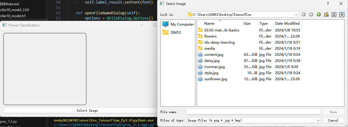
运行代码会打开UI界面, 点击下方Select Image图片选择要预测的图。

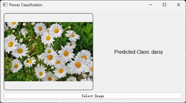
选择图片后会在左侧框内显示, 后台会根据模型进行预测,并返回结果.
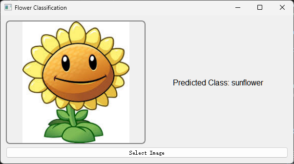
可以看到结果是准确的。

  • Author:

    slacr_

  • Copyright:

  • Published:

    January 19, 2024

  • Updated:

    January 19, 2024

Buy me a cup of coffee ☕.

1000000